Sequence Page
NMR Sequence Definition
The Sequence page in TQT Nuclei provides users with a flexible platform to design and customize NMR experiments. This page supports two powerful methods for creating experiments, catering to both users who prefer coding and those who favor a more visual approach. Below is an overview of the key features and functionality:
Python Code Mode - Code View
In this mode, users can create NMR sequences by directly writing Python code within the application. The code defines the experimental sequence and parameters, and the application interprets the Python script to generate the desired NMR sequence.
LSP Server Integration: To assist users while writing code, the application integrates an LSP (Language Server Protocol) server. This feature offers real-time suggestions and autocompletion for user input, making coding faster and easier. Users will receive helpful hints, shortcuts to local functions, and error checking while writing their experiment scripts.
This mode is ideal for advanced users who are comfortable with coding and want fine control over their experiment parameters.
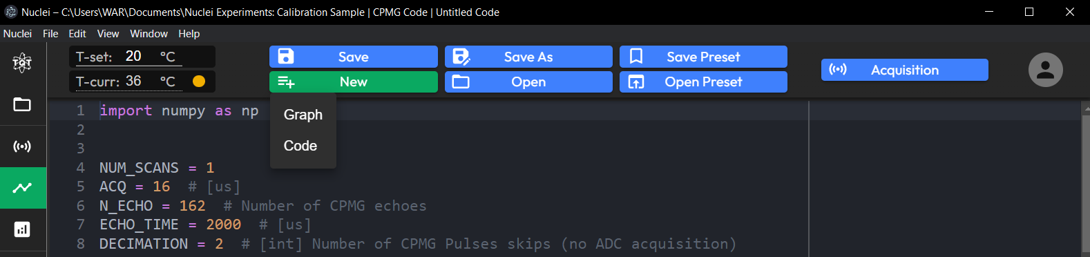
Graphic Nodes Mode - Graph View
For users who prefer a visual approach, the Graphic Nodes Mode allows for the construction of NMR experiments using graphical elements. In this mode, users can drag and drop pre-configured nodes to build an NMR sequence without needing to write code. The following types of nodes are available:
Pulse Node: Represents a radiofrequency (RF) pulse in the experiment.
Silence Node: Represents a delay (τ) or silence period between pulses.
ADC Node: Controls data acquisition during the sequence.
Cycle Node: Allows for looped execution of the experiment, enabling repeated pulse sequences.
Users can assemble these nodes in the lower part of the page on a grid, which serves as the workspace for building the sequence. Each node can be edited and configured to meet the specific needs of the experiment.
- Visual Sequence Representation
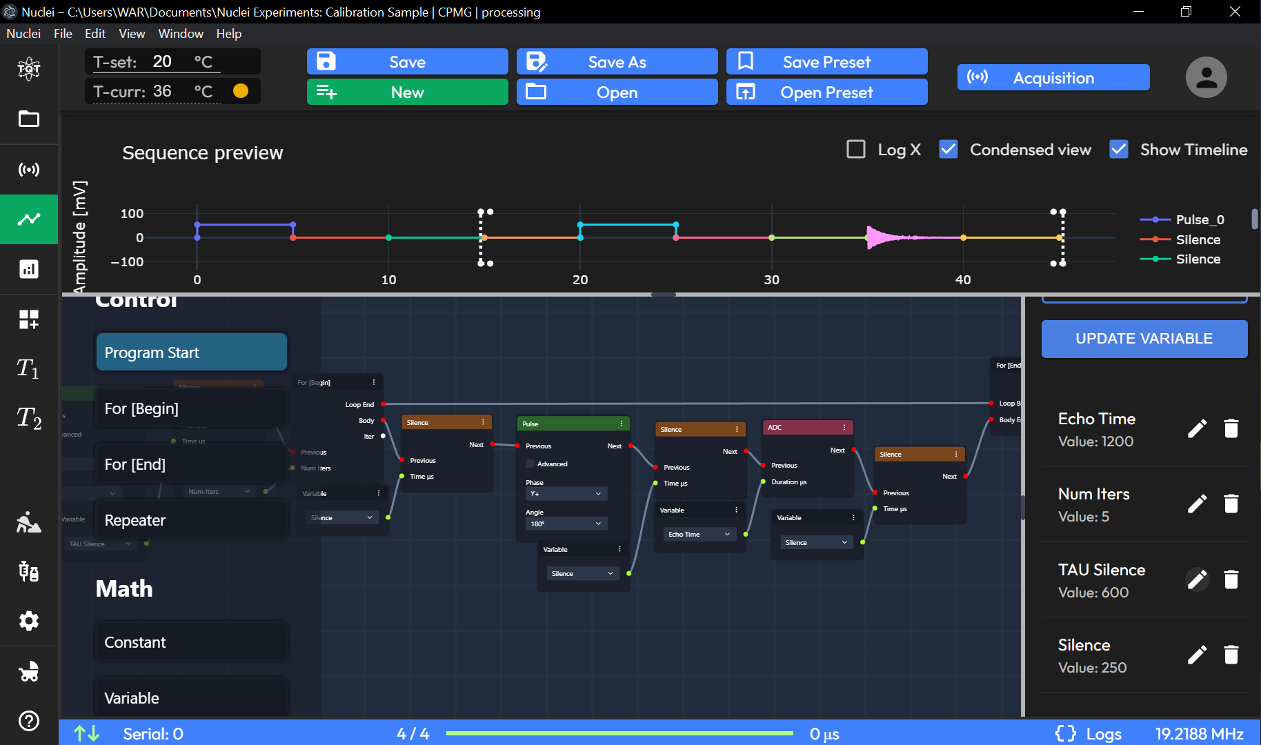
The upper part of the Sequence page provides a visual representation of the NMR sequence. This is displayed in a familiar format for users, showing rectangular pulses, delays, and acquisition windows in the style typically seen in NMR textbooks. The visual representation updates dynamically as users build or modify their experiment, allowing them to see how the sequence is structured in real-time.
- User Variables Panel
At the bottom of the page, there is a panel for inputting and editing user-defined variables. This section allows users to define and adjust parameters such as pulse lengths, delays, and acquisition times. These variables can be referenced in either the Python code or the graphic nodes to create dynamic and customizable experiments.
The Sequence page empowers users to create highly customizable NMR experiments through two different approaches, making it suitable for both coding-savvy users and those who prefer a more visual interface. Whether through Python scripting or node-based design, users have full control over the structure and execution of their NMR sequences.
Code View (Script-Based Definition)
Code Editor: Allows users to define the NMR sequence in Python code. This includes settings for various parameters such as
N_SCANS,ECHO_TIME,ECHO_WIDTH, and acquisition configurations.
Hardware related function from SB45 library:
Pulse: NMR excitation pulses (x+, x-, y+, y-).
Silence: Time between pulses in microseconds.
ADC: Width of the echo, used for capturing the shape of the signal.
Parameters are defined with comments for clarity and can include elements such as:
N_SCANS: Number of scans for the experiment.
ECHO_TIME: Time between pulses in microseconds.
ECHO_WIDTH: Width of the echo, used for capturing the shape of the signal.
Users can customize these parameters directly in the code to create specific NMR sequences.
Graph View (Visual Sequence Editor)
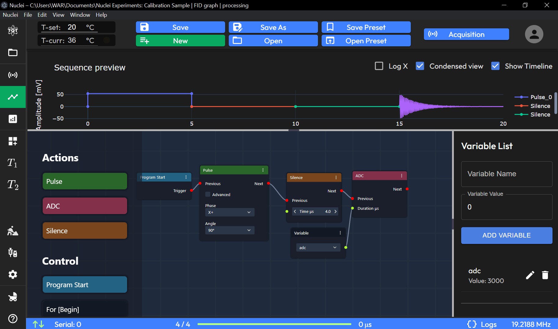
Sequence Preview Graph: Visualizes the sequence timeline, plotting amplitude (mV) over time (µs). Key sequence elements, such as pulses and silence periods, are shown along the timeline.
Log X (Checkbox): Logarithmic scale for the X-axis.
Condensed View (Checkbox): Provides a simplified view of the sequence.
Show Timeline (Checkbox): Displays the timeline for sequence events.
Graph View Mode - Basic Nodes Overview
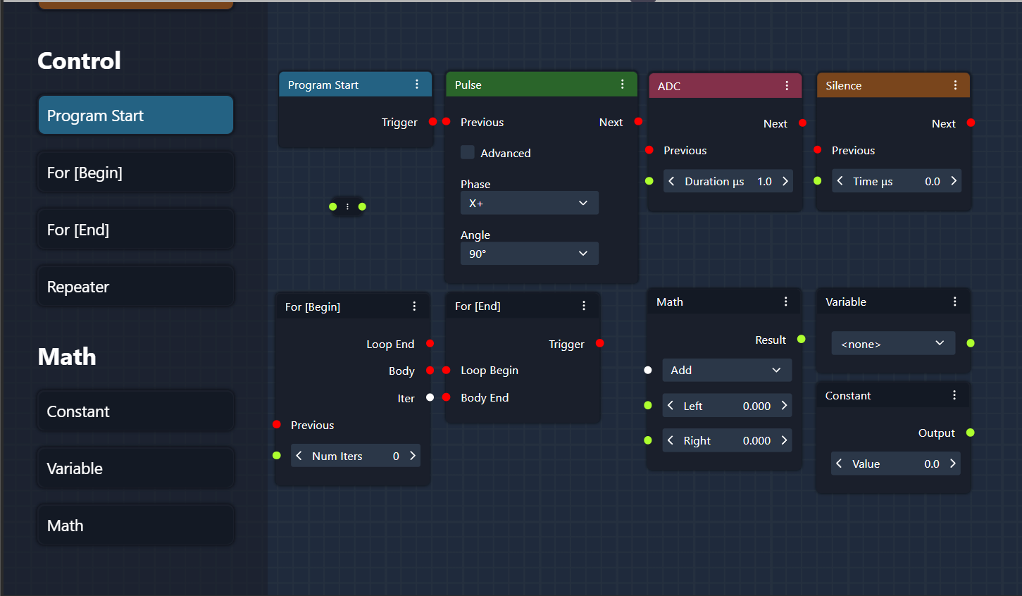
In Graph View Mode on the Sequence page, users can design NMR experiments using a graphical interface by arranging and connecting nodes that represent different elements of the sequence. Below is a description of the basic nodes available:
1. Pulse Node
The Pulse Node represents a radiofrequency (RF) pulse within the NMR sequence. This node allows users to define the characteristics of the pulse, such as:
Duration: The length of the pulse in microseconds or usage of pre-defined values obtained from Duration tuning (see Device Setup).
Amplitude [settings]: The strength of the RF field.
Phase: The phase of the pulse in degrees.
These parameters can be adjusted to fit the experiment’s needs, and the pulse can be connected with other nodes to create complex pulse sequences.
2. ADC Node
The ADC (Analog-to-Digital Converter) Node is responsible for data acquisition during the experiment. When this node is activated in the sequence, it triggers the system to collect signal data from the sample. The ADC node is typically placed after a series of pulses and delays to capture the response of the nuclei.
Acquisition Duration: Defines how long the system should collect data.
Sampling Rate [settings]: Controls the frequency at which data points are captured.
3. Silence Node
The Silence Node represents a period of delay (τ) or dead time in the experiment, where no RF pulses or data acquisition occurs. This node is often used to space out pulses in a sequence and allows spins to evolve before the next pulse or acquisition. The user can define:
Duration: The length of the silence period.
4. Program Start Node (Base Sequence Start Node)
The Program Start Node is the entry point of the sequence and defines where the NMR experiment begins. Every sequence must start with this node, as it sets the initial conditions for running the experiment. It connects to the first pulse, silence, or acquisition node to start the process.
5. For [Begin] Node
The For [Begin] Node marks the beginning of a loop within the sequence. Loops are used when the same sequence of operations needs to be repeated multiple times. Users can define:
Number of Iterations: How many times the enclosed sequence should be repeated.
This node is used in conjunction with the For [End] Node to create a looped structure.
6. For [End] Node
The For [End] Node marks the end of a loop. It connects to the For [Begin] Node and defines the boundaries of the repeated sequence. All nodes between For [Begin] and For [End] are executed for the specified number of iterations.
7. Repeater Node
The Repeater Node functions similarly to a loop but is more flexible and often used for repeating a segment of the sequence with different variable inputs or conditions. It can be used to automate the repetition of a certain experiment while changing parameters such as phase or delay.
8. Math: Constant Node
The Math: Constant Node is used to define a fixed value that can be referenced in other parts of the sequence. For example, if a constant pulse duration or delay is needed throughout the sequence, the value can be defined here and linked to relevant nodes.
9. Math: Variable Node
The Math: Variable Node allows users to define a changeable parameter. This variable can be referenced and adjusted at various points within the sequence, allowing users to create dynamic sequences where parameters change between iterations or loops.
10. Math: Math Node
The Math: Math Node performs mathematical operations on variables or constants defined in the sequence. It allows users to create formulas and calculations that dynamically adjust the sequence parameters based on experimental needs. Operations such as addition, subtraction, multiplication, or division can be applied.
These basic nodes provide users with building blocks to create flexible and customizable NMR sequences, either by using straightforward operations or by combining nodes into more complex experimental designs.
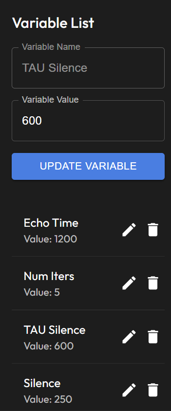
Variable List
Variable Management Panel: Allows the user to define and manage variables used in the sequence, such as
Variable NameandVariable Value.
ADD VARIABLE: Adds a new variable to the sequence for use in different blocks.
EDIT VARIABLE: Edits any created variable in different blocks.
DELETE VARIABLE: Delete any created variable.
Both the code view and the graph view allow users to define NMR sequences with flexibility. Users can switch between views depending on their preference for script-based or visual sequence configuration.
Preset Examples
See following example of the possible logic that could be executed at Sequence Page.
CPMG Code Sequence Page Preset
 1    NUM_SCANS = 1
 2    ACQ = 16  # [us]
 3    N_ECHO = 162  # Number of CPMG echoes
 4    ECHO_TIME = 2000  # [us]
 5    DECIMATION = 2  # [int] Number of CPMG Pulses skips (no ADC acquisition)
 6
 7
 8    def _build_sequence(acq: float, decimation: int,
 9                        n_echo: int, echo_t: float):
10
11        p_90 = DeviceSettings.p90_us
12        p_180 = DeviceSettings.p180_us
13        et = echo_t / decimation
14
15        decimation_sequence = [
16            [Pulse("y-", 180), Silence(et - p_180)]
17            for _ in range(max(0, decimation - 1))
18        ]
19
20        sequence = [
21            Silence(100),
22            Pulse("x+", 90),
23            Silence(et / 2 - p_90 / 2 - p_180 / 2),
24            Cycle(
25                n_echo,
26                [
27                    Pulse("y-", 180),
28                    Silence(et / 2 - p_180 / 2 - acq / 2),
29                    ADC(acq),
30                    Silence(et / 2 - p_180 / 2 - acq / 2),
31                    *[action for step in decimation_sequence for action in step],
32                ],
33            ),
34            Silence(13),
35        ]
36        return sequence
37
38
39    def wobble(acquisition_time: float, n_scans: int, n_echo: int,
40            decimation: int, echo_t: float) -> NMRSpectrum | None:
41
42        amplitudes = []
43        sequence = _build_sequence(
44            acquisition_time, decimation, n_echo, echo_t)
45        # duration = self.runner.estimate_duration(sequence)
46        seq_null = DeviceSettings.p90_us + 100
47
48        for i in range(n_scans):
49            # self.runner.report_progress(i, n_scans, duration)
50            pts_signal, _ = run_sequence(
51                sequence, dry_run=True, seq_null=seq_null, report=False)
52
53            amplitudes.append(np.abs(pts_signal.amplitudes))
54
55            signal = Signal(pts_signal.time_points / 1e3, np.mean(amplitudes, 0))
56            # self.backend.frontend.TunePlotT2Signal(Encoder(signal))
57
58        start_i = np.abs(signal.amplitudes).argmax()
59        signal.time_points = signal.time_points[start_i:]
60        signal.amplitudes = signal.amplitudes[start_i:]
61
62        return signal
63
64
65    # Fitting
66
67    def t1_exp_model(x, a, b, c):
68        return a * np.exp(-x / b) + c
69
70
71    curve = wobble(ACQ, NUM_SCANS, N_ECHO, DECIMATION, ECHO_TIME)
72    plot(curve)
73
74    [scale, T1, y0], err = fit_model(curve, t1_exp_model)
75    print(f"{scale=}, {y0=}, {T1=}, {err=}")
76
77    annotate(Signal(
78        curve.time_points,
79        t1_exp_model(curve.time_points, scale, T1, y0)
80    ), name="T2 Fit")
81
82    # save_custom(curve)
83    save(curve)
T1 Inversion Recovery Code Sequence Page Preset
 1    ACQ = 10  # [us]
 2    ANTICIPATED_TIME = 10000  # [us] Curve Start time
 3    N_POINTS = 16  # [int]
 4    PERIOD = 750000  # [us] Curve End time
 5    NUM_SCANS = 1  # [int]
 6
 7
 8    def wobble(tau_2: float) -> NMRSpectrum | None:
 9        p_90 = DeviceSettings.p90_us
10        p_180 = DeviceSettings.p180_us
11        tau_1 = DeviceSettings.ring_us
12        seq_null = p_90 + p_180 + tau_1 + tau_2 + 120
13
14        sequence = [
15            Silence(120),
16            Pulse('x+', 180),
17            Silence(tau_2),
18            Pulse('x+', 90),
19            Silence(tau_1),
20            ADC(ACQ),
21            Silence(tau_1),
22        ]
23        sig, spec = run_sequence(sequence, seq_null=seq_null)
24
25        amps = np.abs(sig.amplitudes)
26        return np.mean(amps[2:16])
27
28
29    def record():
30        x_start = ANTICIPATED_TIME
31        step = np.exp(np.log(PERIOD / x_start) / (N_POINTS - 1))
32        sig_amps = []
33
34        for _ in range(NUM_SCANS):
35            xx, yy = [], []
36            x = x_start
37
38            for i in range(N_POINTS):
39                xx.append(x / 1000)
40                yy.append(wobble(x))
41                x *= step
42
43                sig_amps.append(yy)
44
45        return Signal(np.array(xx), np.mean(sig_amps, 0))
46
47
48    def t1_exp_model(x, a, b, c):
49        return a * np.exp(-x / b) + c
50
51
52    curve = record()
53    plot(curve)
54
55    [scale, T1, y0], err = fit_model(curve, t1_exp_model)
56    print(f"{scale=}, {y0=}, {T1=}, {err=}")
57
58    annotate(Signal(
59        curve.time_points,
60        t1_exp_model(curve.time_points, scale, T1, y0)
61    ), name="T2 Fit")
62
63    # save_custom(curve)
64    save(curve)
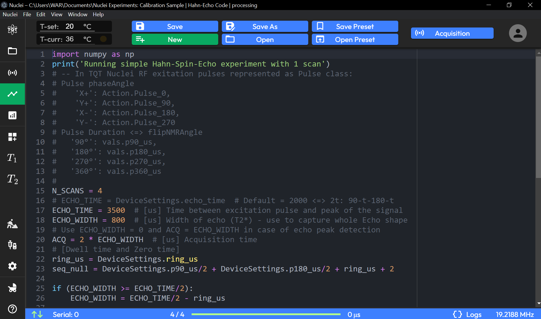
Hahn-Echo Code Sequence Page Preset
1 print('Running simple Hahn-Spin-Echo experiment with 1 scan')
2
3 N_SCANS = 4
4 # ECHO_TIME = DeviceSettings.echo_time # Default = 2000 <=> 2t: 90-t-180-t
5 ECHO_TIME = 3500 # [us] Time between excitation pulse and peak of the signal
6 ECHO_WIDTH = 800 # [us] Width of echo (T2*) - use to capture whole Echo shape
7 # Use ECHO_WIDTH = 0 and ACQ = ECHO_WIDTH in case of echo peak detection
8 ACQ = 2 * ECHO_WIDTH # [us] Acquisition time
9 # [Dwell time and Zero time]
10 ring_us = DeviceSettings.ring_us
11 seq_null = DeviceSettings.p90_us/2 + DeviceSettings.p180_us/2 + ring_us + 2
12
13 if (ECHO_WIDTH >= ECHO_TIME/2):
14 ECHO_WIDTH = ECHO_TIME/2 - ring_us
15
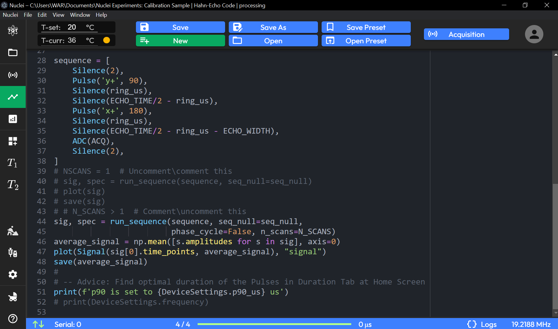
16 sequence = [
17 Silence(2),
18 Pulse('y+', 90),
19 Silence(ring_us),
20 Silence(ECHO_TIME/2 - ring_us),
21 Pulse('x+', 180),
22 Silence(ring_us),
23 Silence(ECHO_TIME/2 - ring_us - ECHO_WIDTH),
24 ADC(ACQ),
25 Silence(2),
26 ]
27 # Pulse phaseAngle
28 # 'X+': Action.Pulse_0,
29 # 'Y+': Action.Pulse_90,
30 # 'X-': Action.Pulse_180,
31 # 'Y-': Action.Pulse_270
32 # Pulse Duration <=> flipNMRAngle
33 # '90°': vals.p90_us,
34 # '180°': vals.p180_us,
35 # '270°': vals.p270_us,
36 # '360°': vals.p360_us
37 #
38 sig, spec = run_sequence(sequence, seq_null=seq_null,
39 phase_cycle=False, n_scans=N_SCANS)
40 average_signal = np.mean([s.amplitudes for s in sig], axis=0)
41 plot(Signal(sig[0].time_points, average_signal), "signal")
42 save(average_signal)
43 #
44 # -- Advice: Find optimal duration of the Pulses in Duration Tab at Home Screen
45 print(f'p90 is set to {DeviceSettings.p90_us} us')
46 # print(DeviceSettings.frequency)